Whooosh, and another semester zooms by

Crikey, I sure haven’t posted!

Some news and reflection:

This last semester in regular Statistics is the first time I have taught a class for the second time. I went back and forth the whole time in my off-the-cuff assessment of whether it was any better. Easier, sure: I definitely was able to use material from last year. But did it take any less time? No. And most important, was I any better at paying attention to the students? There I’m not sure; I really felt, a lot of the time, that I was neglecting the most experienced students while I helped those who were having the most trouble. Or, more generally, that despite getting better as a teacher, there are many ways in which I suck. This is not as self-flagellatory as it sounds (as Walter Brennan used to say, “no brag, just fact”) but rather the continuing realization that this path requires continuing improvement.

All of which is alleviated somewhat by seeing the student work, especially on the semester projects. Everybody can improve, of course, but they were, in general, kind of wonderful.

Mathematical Practices

Okay, everybody, check out Mimi’s post from today. It has a links to two documents, just made available: a rubric and a supplement to the rubric about those elusive Standards for Mathematical Practice in the Core Standards.

You have seen the list of habits-of-mind-y phrases:

Mathematical Practices

1. Make sense of problems and persevere in solving them.
2. Reason abstractly and quantitatively.
3. Construct viable arguments and critique the reasoning of others.
4. Model with mathematics.
5. Use appropriate tools strategically.
6. Attend to precision.
7. Look for and make use of structure.
8. Look for and express regularity in repeated reasoning.

One could quibble about details, but it’s a darned good list. The standards doc itself describes them for two pages, then goes on to spend its bulk delineating content. The Core peeps clearly thought the practices were important, but there’s not a lot of guidance that would lead to (imagine!) assessments of habits of mind.

And if we care about them, we should assess them. Right?

So a rubric is especially welcome. What’s amazing about it is that it’s not directed at the students’ behaviors, but rather at teachers and the tasks we write. It’s interesting and refreshing, and a really good piece of work. Bravo!

Should we have standards for mechanical skills?

A couple posts ago, I said that I liked my learning goals (i.e., standards) pretty much, but that they were really different from one another.

But shouldn’t standards be kind of similar in size and type of material? Maybe not.

Let’s assume that we should assess what we care about, and that standards represent pretty directly what we assess. So if I care about different kinds of things, I should try to write standards that reflect that. I think I was pretty successful at making some standards that fit content-y topics and others that demand big, broad, synthesis—at least for a noob—but I’m puzzled about skills.

I do care that students know how to use Fathom to do particular things.

This is because I believe that doing those things with reasonable fluency will help them understand the content.

Still, Fathom proficiency is not content. So should I assess only the desired result?

On the other hand, some “Fathom” standards give some kids a chance to master something.

As an example, let’s look at two “mature” learning goals. That is, they’re from late in the course when I had gotten better, or at least faster:

27 Fathom: Three-Collection Simulations (scrambling and measures)

• 27.1 Given an appropriate situation (comparing some variable across two groups) define a sensible measure to describe the observed difference; compute that test statistic.
• 27.1.1 For quantitative variables, use measures of center (and probably difference or ratio)
• 27.1.2 For categorical variables, the measures probably use proportion or count
• 27.2 Create a sampling distribution of that statistic using scrambling
• 27.3 Use that distribution and the test statistic to find the empirical probability that the test stat could arise if there were no association between the group membership and the variable under study.

28 Basics of Inference

• 28.1 Understand these terms as applied to any of the Fathom simulations we have been doing:
• 28.1.1 Sampling distribution
• 28.1.2 Test statistic
• 28.1.3 P-value
• 28.1.4 Null hypothesis
• 28.2 Given an analysis with a sampling distribution and a test statistic,
• 28.2.1 Calculate the P-value
• 28.2.2 Understand that the P-value is the probability that—if the null hypothesis were true—you would get a value as extreme as the test statistic
• 28.2.3 Correctly interpret a low P-value (e.g., it’s implausible that this value is due to chance)
• 28.2.4 Correctly interpret a high P-value (e.g., we can’t rule out chance as the reason for this value)

So LG27 is just skills. Complicated skills, but skills nevertheless. LG28 is the meat of inference. My gut tells me to keep them both, and keep them separate. But I’d be interested in what others think (including a Tim with more experience…)

In the cold light of morning: Interestingly, LG27 (above) is not just mechanical skills; part of the point is making the connection between a real-life situation and an appropriate statistical technique, especially including developing the measure—the number that tells how big the effect is that you have noticed. And LG28 is not just the meat of inference: 28.1 specifically is talking about applying terms in the context of a Fathom simulation. Does that make it mechanical or too software-specific? I don’t think so. Looking back, I think I wrote it that way because I believe that if students can do this, they actually understand how inference works. Fathom itself uses none of these terms, so identifying them in the Fathom context means you have to understand them pretty thoroughly.

Having said that, I see that the first three are really different from the fourth, “null hypothesis.” They don’t actually exist outside an analysis, so you can’t really talk about a sampling distribution (say) without imagining an analysis, probably on a computer, or actually doing one. We can talk about null hypothesis without any of that, though; it arises directly out of a situation and noticing something of interest.

Which may explain why it made sense to me to do exercises where I had students write the null hypothesis for a number of situations.

Fantasy and Reality in Inference

In which he describes his approach to inference.

The null hypothesis is never true.

I guess I knew this at some level, but I never really got it till this Spring. Then it hit me that this was worth telling students. (Can I get them to discover it? Maybe.)

Let me back up a bit and approach it from the direction of Aunt Belinda.

Aunt Belinda: A Touchstone Situation

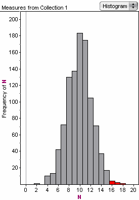
1000 simulations of 20 coin flips. Seven of them (selected, in red) have 16 or more heads.

Aunt Belinda claims to have power over flipping coins. She takes 20 nickels and throws them into the air. When they land, there are 16 heads. How should we interpret this result?

I want kids to learn to ask, “is it plausible that the coins are fair and Belinda has no special powers?” and realize that they can answer that question by flipping 20 fair coins over and over again, and seeing how often you get 16 or more heads.

Setting aside a lot of other discussion (no, she refuses to do it again) and what I hope is obvious pedagogy (the first time you see this, everybody gets 20 actual coins and has to do it a few times, chasing the rollers all over the classroom), we get Fathom to do the simulation because it saves so much time. Early on, I posted a graph showing the result of a whole lot of simulated 20-coin events, and reproduce it here.

At this point, we confront the basics of statistical inference. (These are also the bullet points in one of my learning goals, a.k.a. standards.)

• P-value. Seven out of 1000. Is it plausible? Students need to distinguish plausible from possible. Ideally, we also set some plausibility limit on this empirical P-value (which is what this 0.007 is after all) that depends on the circumstance and how willing you are to be wrong (oooh! Type I errors!). This last year, I mentioned that a lot but basically punted and explained that an orthodox reasonable value was 0.05.
• The null hypothesis is that the coins are fair, and there are no special powers. Articulating a null hypothesis is important. I began my discussion of the null by saying that it’s often the dull hypothesis: the situation when nothing of interest is going on.
• The sampling distribution is the one in the picture: repeated results from trials where the null hypothesis is true. They are not the same because random events come out differently even when the coins are fair.
• The test statistic is 16 heads out of 20. It’s what you compare to the sampling distribution to assess whether the result is plausible.

We then draw a conclusion, in this case, to reject the null hypothesis. That is, we think that something—we’re not sure what—is interefering with a fair toss of the coins. And we admit that it is possible (but not plausible) that we’re wrong and the coins are in fact fair.

What goes wrong? 

What Went Right

Yikes. Another couple months. And a lot has happened: I experienced senioritis firsthand, our house has been rendered uninhabitable by a kitchen remodel (so we’re living out of suitcases in friends’ spare rooms), and my first year of actually teaching stats has drawn to a close.

It is time to reflect.

My tendency is to flagellate myself about how badly I suck, so (as suggested by Karen E, my brilliant and now former assistant head of school, we’ll miss you, Karen!) let me take a deep breath and report first on what seemed to work. Plenty of time for self-flagellation later.

Resampling, Randomization, Simulation, and Fathom

The big overarching idea I started with—to approach inferential statistics through resampling à la George Cobb—worked for me and for at least some students. It is not obvious that you can make an entire course for these students with randomization as the background. I mean, doing this is mapping an entirely new path through the material. Is it a good path? I’m not certain, but I still basically believe it is.

To be sure, few of my students got to the point where they automatically chose the right technique at every turn. But they did the right thing a lot, and most important for me, I never had to leave them in some kind of mathematical dust where they made some calculation. For example, (and I may be wrongly proud of this) we got through an entire year of statistics without introducing the Normal distribution. This may seem so heretical to other teachers, it deserves a post of its own. Later. The point here is that no student ever was in a position of calculating NormalCDF-of-something and not understanding what it really meant.

Did they perform randomization tasks and not really understand? Sure. But when they did, they did so “closer to their data,” so they had a better chance to fix that non-understanding. They didn’t rely (for example) on the Central Limit Theorem—which, let’s face it, is a black box—to give them their results.

Fathom and Technology

Fathom was a huge suggess throughout. It was great to be able to get them all the software and assign homework in Fathom. They enjoyed it, and really became quite adept at using the tool.

One big question was whether they would be able to use the “measures” mechanisms for creating their own simulations. Basically, they can. It’s a big set of skills, so not all of them can do everything we covered, but in general, they understand how to use the software to implement randomization and simulation techniques. This goes hand in glove with actually understanding what these procedures accomplish.

We also became more and more paper-free as the year went on, setting and turning in more and more assignments as pdfs. The “assignment drop box” wasn’t perfect, but it worked well enough.

Starting SBG

I decided to try standards-based grading, at least some local version of it, in this first year. On reflection, that was pretty gutsy, but why wait? And it worked pretty well. Most importantly, students overwhelmingly approved; the overall comment was basically, “I like knowing what’s expected.” Furthermore—and this may be a function of who the kids were more than anything else, bit I’ll take it—there was hardly any point-grubbing.

It is also satisfying to look over my list of 30-ish standards and see that

• They largely (but not completely) span what I care about.
• They set standards for different types of mastery, ranging from understanding concepts to using the technology to putting together coherent projects.

They need editing, and I need to reflect more about how they interact, but they are a really good start.

Flipping and Video

At the semester break, I decided to take a stab at “Flipping the Classroom.” This was a big win, at least where I used it most—in giving students exposition about probability.

There is a lot that can go wrong with videos as instruction (the Khan brouhaha is a good example; see this Frank Noschese post for a good summary of one view) and I want to explore this more. But the basic idea really works, and the students recognized it: if it’s something you would lecture about, putting it on the video has two big plusses:

• They can stop and rewind if they don’t get it
• You can do it over til you get it the way you want. No more going back and saying, “when I said x it wasn’t quite right…”

My big worry is that if I assign videos as homework, hoping to clarify and move on in class, that the lazy student may watch, but will blow off thinking, assuming that they can get me to cover it again. I need to figure out a non-punitive way around that problem; or maybe it’s not so bad simply to be able to use class time for the first repetition…

Some Cool Ideas

Besides these esssentially structural things, I had some frankly terrific ideas during the year. Some I have mentioned before, but let me list just four, just as snippets to remind me what they were; later if I get to it I’ll elaborate:

• Using sand timers and stopwatches to explore variability.
• Going to the nearby freeway overpass to sample cars.
• Using the school’s library catalog to do random sampling.
• Going to the shop to make dice that were not cubes.

There were other curricular successes such as using old material from Data in Depth—particularly the Sonatas—for work during the first semester.

Wonderful Kids

I can’t say enough about how much I appreciate the students. Again, I could do better at helping create a really positive class culture, but they did pretty damned well on their own. They got along well, took care of each other, exchanged good-natured barbs, were good group members and contributors.

Even the most checked-out seniors, already accepted into college and having reached escape velocity: they may not have worked very hard outside of class, and assignments may have slipped, but in class they were engaged and still learning. And some juniors did strong, strong work that will make writing college recs easy next year.

And I got a couple of those letters—teachers, you know the ones I mean—that make it worth the effort.

So all in all, a good year. Much to improve, yes. But it’s worth savoring what went right.

Inference for Slope: Fathom How-to

Too long again since the last post.

Here we have something interesting that’s outside the narrative thread. On the AP Stat list serve, Chris Talone asked this question:

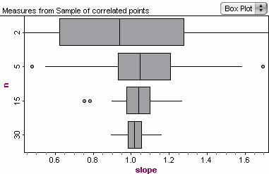
Is there a way to set up a Fathom simulation to illustrate how the slope of a line of best fit will vary when choosing ordered pairs from a population of ordered pairs?  My students are having a hard time understanding the purpose of the linear regression t-interval and the linreg t-test.  I would like for them to see how the slope can vary depending on the sample of points chosen.  Ideally, I’d like to set up a population of ordered pairs, graph a scatterplot and find the line of best fit for the population, then have Fathom randomly select 2, 5, or 7 of those ordered pairs, graph a scatterplot of the sample chosen, find the line of best fit for the sample chosen, and also plot the sample slope on a dot plot, and then repeat many many times….

I posted a response there, but we can’t give illustrations. We can here! This is where we’re heading:

We've sampled 100 times with sample sizes of 2, 5, 15, and 30 (the size of our original collection). A box plot is good for comparing.

How do we do this in Fathom? Read on…

Never mind winning the race. Are we on the right track?

It’s another crisis of confidence in stat-teacher land. It’s actually not as bad right now as it was over the last week, all thanks for the improvement be to wonderful students. But still. I feel like Ralph Rackstraw in HMS Pinafore:

…in me there meet a combination of antithetical elements which are at eternal war with one another. Driven hither by objective influences — thither by subjective emotion — wafted one moment into blazing day by mocking hope — plunged the next into the Cimmerian darkness of tangible despair, I am but a living ganglion of irreconcilable antagonisms. I hope I make myself clear…

No? To me neither. In any case, the end of the third quarter fast approaches, and we’re battering away at the Gates of Inference. Will we get inside in time to do anything with it?

I’ve been really pleased with this semester’s arc so far. Staying empirical, mostly. Starting with some hands-on probability, learning to simulate in Fathom, then building up the simulation skills while addressing increasingly realistic and relevant problems. And I like my choice of aiming for “scrambling” situations; we’re now doing randomization tests with student-constructed measures to assess group differences in settings that the students choose. They don’t know they’re called randomization tests, and we’re picking strong associations (so P is generally ≤ 0.001), so everything is obvious, but they are mostly doing them. We’ve been saying the inference-y words a lot without adding the principles to the learning goals (yet), so this is mostly mechanical—but the students are gradually getting the idea.

So it seems good! Robin Lock even commented! More videos got made! And I have yet to mention the Normal distribution, which I view as a very good thing. I mean, imagine: actually understanding the basics of stats without having to break out the Normal.

But then two things happened:

• I read parts of a few chapters in Workshop Statistics (Rossman, Chance, and the same Lock)
• I started realizing how much else I wanted to get to

As to the first, nothing is quite so depressing as seeing that somebody else has done a much better job of organizing a bunch of material. Of course, they take a more traditional path though this thicket (they do include the Normal; then again, theirs is a college class), but they have a dizzyingly terrific set of activities that build well on one another. So I wonder if I should have bitten the bullet and bought a set of these—and hewn closely to their curriculum instead of going my own way on this.

And as to the second, I know I want to see if I can use this randomization approach on other forms of inference, both tests and estimates. But I also want them to have time for projects and a lot else, like expected value and gambling. And, save me, but I worry how much I need to expose them to more orthodox stats approaches, so that later when they tell a professor they took stats  in high school and the prof asks, “well, is this a t situation, or is this where we use chi-square?” they will actually be able to answer.

It all combines to fill me with doubts and feelings of total doofusism, that I have stupidly led these students into some box canyon where they can’t quite understand something that, if they did, would not quite be enough to get the big picture I think is so important. I have not described this well, but it’s a start. Another whole big slab of self-loathing comes from bad use of time and lousy follow-through.

Meanwhile, the scrambling video. From way last month. This one uses ScreenFlow instead of Camtasia:

 

Analyzing Two Dice

Back at the beginning of the semester, I said that I wanted kids to get a picture in their heads about adding two dice. Here are some (belated) results.

On the first quiz, way back in January, I asked this question:

Aloysius says, “if you roll two dice and add, the chance that you get an even number is P(even) = 0.5 because half of all whole numbers are even.”

Use an area model to help show that he’s right that P = 0.5, but explain why his reasoning is wrong.

I expected students to add up the various probabilities for sums of 2, 4, 6, 8, 10, and 12—(1/36 + 3/36 + 5/36 + 5/36 + 3/36 + 1/36)— get 18/36 and say it was 1/2. How silly I was. They were much more creative.

I also hoped they would say that the reasoning was bad because the numbers are not equally likely. How silly I was.

Right Answers

Anyhow, some diagrams. Click to enlarge. First, the most popular. I hadn’t anticipated the “checkerboard” aspect of the area diagram and how easy it would be to see that half of the (equally-likely) combinations were even. It also tempts one to make an analogous problem with five-sided dice:

Here is the diagram; the legend is next.

The legend and explanation for the "checkerboard" response.

But then, several students used this kind of diagram, which is kind of brilliant and totally unexpected (by me at least):

A different approach: this student reasons about the sums of even and odd numbers rather than from the canonical diagram.

Wrong Answers

Of course, there were still islands of trouble, for example:

Here, the student does not get how the area model works despite having watched the videos.

We also have this one; where it come from no one (least of all the student) is sure. I include it for all you teachers out there who will nod and say, “yup, you never know what you’re gonna get.” Remember: click to enlarge.

An unusual area model. No one knows why the student used the sizes in the diagram.

What do we make of this? The best thing is that the student at least knew that something was wrong with the diagram, and owned up to it on the paper. This is something I have been asking them to do, and I get it really seldom.

But then, the denominator 441 is in fact the number of little squares in the diagram (21 x 21), but of course 220.5 of them are not colored in; that’s just the number you’d have to have to make the probability 0.5.

So I have an assessment problem. I’m reasonably convinced that the right answers show some level of understanding, but I can’t really tell, from the wrong answers, what’s going wrong.

Parte Deux: Why Aloysius was Wrong

Although most of the diagrams were good, most of the responses to why Aloysius’s reasoning was bad were not. Here’s one that makes me doubt myself to the core:

His reasoning is wrong because you never know what you’re going to roll but you do know that 50% of the possible sums are even but not that you’ll roll an even number/sum 50% of the time.

Here’s one that shows a good observation (but still doesn’t complete the catch):

Aloysius’s reasoning is wrong because in the spread of #s (sums) that you can get, which is 2–12, there are more even #s. What he should have said was that

I don’t know

Then an attempt to use the vocabulary:

The probability of rolling two dice and having an even sum is mutually exclusive…

There were also a handful of non-responses, a handful of good ones, and the rest something like the above. Many were enough longer that I will spare you reading them.

Anyhow, I really like the question in principle, so what should I do about this? On the second quiz, I put in another Aloysius question—I gave them a Fathom simulation with lots of mistakes, and asked them to identify the mistakes and fix them. I think that went better. I will also be insisting on corrections in order to do re-takes to improve the scores on the corresponding learning goals. That will at least force them to confront what went on and think about it again.

But now it’s time for dinner.

Another vid: Fathom simulations with sampling

The classic randomization procedure in Fathom has three collections:

• a “source” collection, from which you sample to make
• a “sample” collection, in which you define a statistic (a measure in Fathom-ese), which you create repeatedly, creating
• a “measures” collection, which now contains the sampling distribution (okay, an approximate sampling distribution) of the statistic you collected.

This is conceptually really difficult; but if you can do this (and understand that the thing you’re making is really the simulation of what it would be like if the effect you’re studying did not exist—the deeply subjunctive philosophy of the null hypothesis, coupled with tollendo tolens…much more on this later), then you can do all of basic statistical inference without ever mentioning the Normal distribution or the t statistic. Not that they’re bad, but they sow confusion, and many students cope by trying to remember recipes and acronyms.

My claim is that if you learn inference through simulation and randomization, you will wind up understanding it better because (a) it’s more immediate and (b) it unifies many statistical procedures into one: simulate the null hypothesis; create the sampling distribution; and compare your situation to that.

Ha. We’ll see. In class, we have just begun to look at these “three-collection” simulations. I made a video demonstrating the mechanics, following the one on one- and two-collection sims described in an earlier post. They are all collected on YouTube, but here is the new one.

Comments welcome.

Making Simulations in Fathom: another scaffold, technical challenges

I’ve posted recently about “flipping the classroom,” the idea of putting the exposition—the lecturing—in little digestible vodcasts to be watched at home, (ideally) leaving more time for discussion, one-on-one work, etc., and (ideally) preventing me from nattering on and boring my students.

In that effort I made a series of vids about probability. Now we’re making simulations in Fathom, exploring empirical probability, and beginning on the road to inference. (We’re avoiding the orthodox terminology for now: don’t tell the students, but they’re simulating the conditions of the null hypothesis in order to compare the test statistics to the sampling distributions they create in the simulations. See the post about randomization.)

It’s going OK, but once you use randomness and make measures, you’re no longer in beginning Fathom. It’s conceptually harder as a whole, and the mechanics of the software inevitably ramp up in difficulty as well. So I’ve made a video that’s all about the mechanics of doing this in Fathom with one and two collections. (The three-collection case is coming…)

You wanna see it? Here it is:

Anyway, in that effort, I thought that the easy-peasy way to make the videos—using Keynote—was not sufficient. So I used Camtasia Studio, which was really fun and worked fine.

I’m looking into ScreenFlow for capture as well, and Vimeo for distribution.

Note: I had trouble for a while with getting the resolution right in YouTube. Coulda sworn that one of the Camtasia presets for YouTube was 480 x 640, but it’s 380 x 640. Text came out looking crummy, like this:

Example from YouTube uploaded at 480 x 640. Note the crummy text.