More about Data Moves—and R

In the previous post (Smelling Like Data Science) we said that one characteristic of doing data science might be the kinds of things you do with data. We called these “data moves,” and they include things such as filtering data, transposing it, or reorganizing it in some way. The moves we’re talking about are not, typically, ones that get covered in much depth, if at all, in a traditional stats course; perhaps we consider them too trivial or beside the point. In stats, we’re more interested in focusing on distribution and variability, or on stats moves such as creating estimates or tests, or even, in these enlightened times, doing resampling and probability modeling.

Instead, the data-science-y data moves are more about data manipulation. [By the way: I’m not talking about obtaining and cleaning the data right now, often called data wrangling, as important as it is. Let’s assume the data are clean and complete. There are still data moves to make.] And interestingly, these moves, these days, all require technology to be practical.

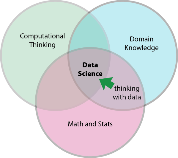
This is a sign that there is something to the Venn diagram definitions of data science. That is, it seems that the data moves we have collected all seem to require computational thinking in some form. You have to move across the arc into the Wankel-piston intersection in the middle.

I claim that we can help K–12, and especially 9–12, students learn about these moves and their underlying concepts. And we can do it without coding, if we have suitable tools. (For me, CODAP is, by design, a suitable tool.) And if we do so, two great things could happen: more students will have a better chance of doing well when they study data science with coding later on; and citizens who never study full-blown data science will better comprehend what data science can do for—or to—them.

At this point, Rob Gould pushed back to say that he wasn’t so sure that it was a good idea, or possible, to think of this without coding. It’s worth listening to Rob because he has done a lot of thinking and development about data science in high school, and about the role of computational thinking.

Aside: Rob tends towards R Studio as his weapon of choice, that is, have students use a real tool, but in a suitably scaffolded environment. There is much to be said for this, but I can imagine a lot of grappling with R’s syntax among many students I have taught; I think it would be better to focus on ideas such as “identifying and looking at a relevant subset of the data” in a more gesture-based environment (e.g., CODAP) and connecting that to the data, the data stories, claims, and questions—and then, later, doing it in code. To be sure, with coding you can do anything. Using CODAP will limit what you can do. But it might expand what you will do, and what you will understand.

We discussed this some more, and he made a great suggestion: see how our nascent “data moves” correspond to what the big dogs in the R world think. Hadley Wickham’s dplyr R package implements a “grammar of data manipulation” with a goal of identifying “the most important data manipulation verbs.” Verbs! These are moves! So: what are dplyr‘s most important verbs?

That’s easy: group_by, summarise, mutate, filter, select and arrange

So let’s start with these.

group_by

Use this function to convert a table into a “grouped” table. You tell R the variable you want to group by, and R separates the table according to the values of that variable. For example, you can group by sex, and subsequent calculations will treat females and males separately.

In the CODAP world,

• If you drag the sex attribute into a graph, the points get colored according to the sex of the cases they represent.
• If you drag the sex attribute to an axis of a graph, the graph separates into two—one for females, one for males—and you see parallel univariate graphs such as dot plots.
• If you drag sex leftwards in the table, CODAP restructures the table hierarchically into sub-tables for females and males, making sex a “parent” attribute. New attributes at that parent level (with values defined by aggregate functions such as mean(height)) have values for each group.

So we see three different takes on grouping. The third is the most general, but arguably the hardest conceptually. Students easily understand coloring points by sex (or by whatever) and don’t get stuck in any syntax trouble.

summarise

“Summarise multiple values to a single value.”

That is, do an aggregate calculation. If we had a table of people with sex and height, a pseudo-r command such as

summarise(group_by(sex), mean(height))

would produce a table showing the mean heights of the two sexes.

As suggested above, in the CODAP world, you would create a new attribute at the “parent” level of a table, and give it that mean(height) formula. On the screen, it would look like this:

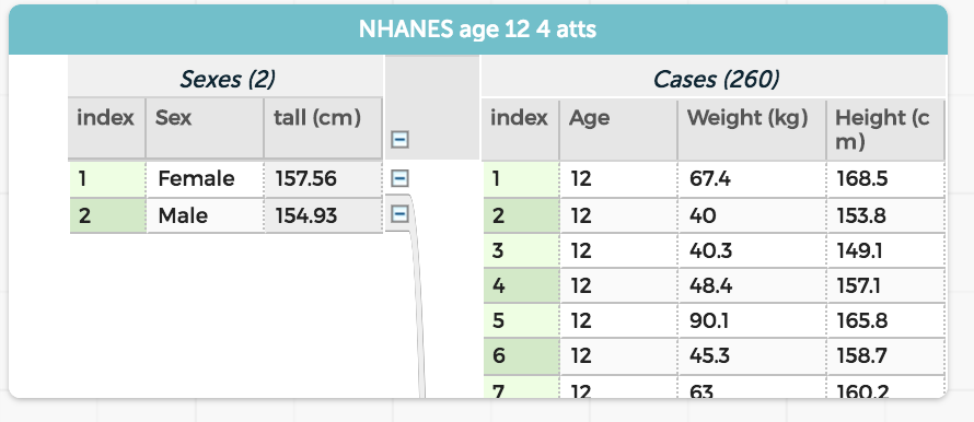
mutate

Use this function to add a new variable to an R table, typically with values computed by a formula. This is something like summarise, but for the case-level data. For example, in the CODAP table above, where height is in centimeters, we could compute it in inches with pseudo-R like this:

mutate(NHANES, Height_in = Height/2.54)

and we would get a new column in the table.

Curiously, CODAP makes no distinction between making an aggregate computation as we did above to compute the mean height and a case-by-case calculation where R uses mutate. In CODAP, whether you want to mutate or summarise, just add a column and write the formula. You must, however, add the column at the right “level” of the hierarchical table to get the result you need. You also need to use a suitable function in your formula; CODAP functions such as mean() or count() produce aggregate values over their group.

filter

“Return rows with matching conditions.”

That is, focus on a subset of the data in R. If we just wanted the mean height of females, we might write:

summarise( filter(NHANES, Sex == "Female"), mean(Height))

The key thing is that the student writes a Boolean expression (Sex == "Female") that represents the subset. And get all the parentheses right. Now, I’m not against learning syntax or how to write a Boolean expression. And in fact, I’m pushing for Boolean-expression filtering in CODAP right now. But it would be great to experience how useful filtering is in order to see why you would ever want to learn that.

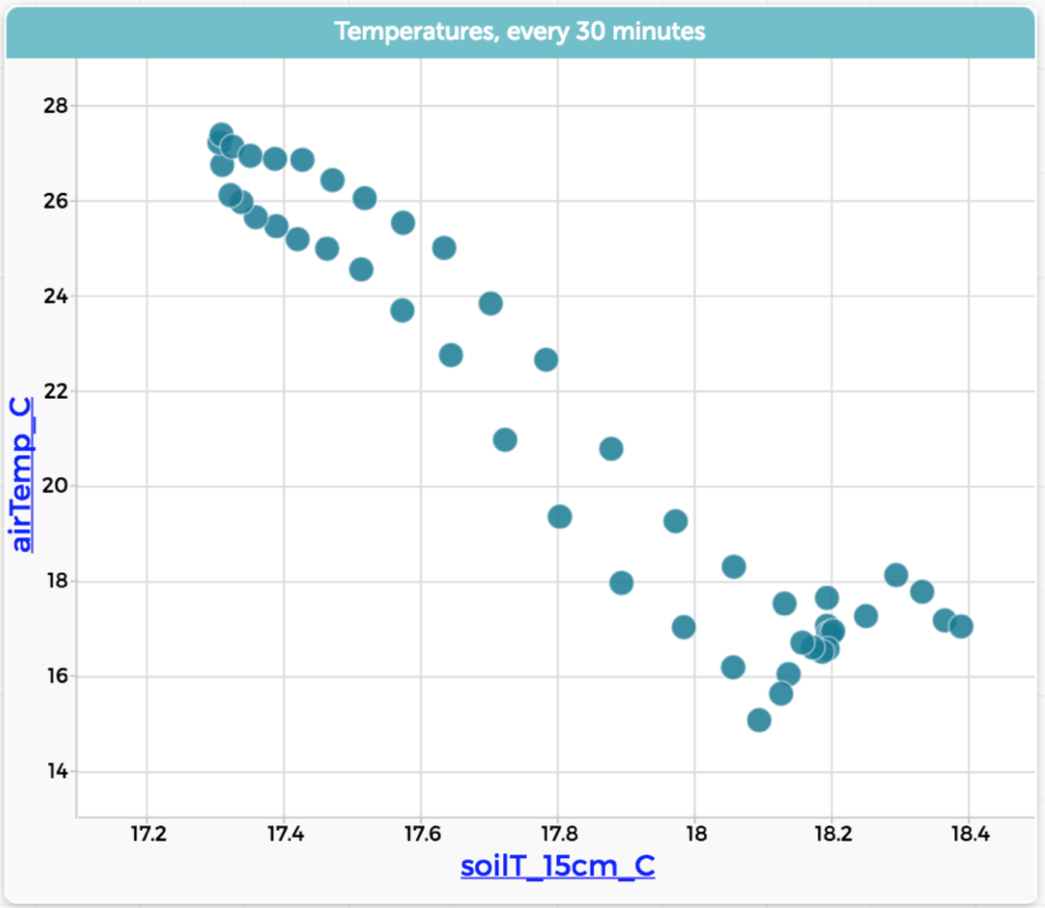
To that end, CODAP lets you filter using selection. That is, you select the cases (in R-speak, “rows”) in any representation of the data—table or graph—and then  ask CODAP to display only the selected cases, or only the unselected ones. Here are data showing soil temperature and air temperature at a site in a California forest. It’s one year of data, taken every 30 minutes:

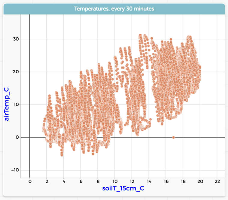
We can see that, in general, the higher the air temperature (vertical axis; maybe it would be better the other way…) the higher the soil temperature. That makes sense, but it’s a lot of data and the details are all mushed together. Now suppose we go to our table and select one day in July:

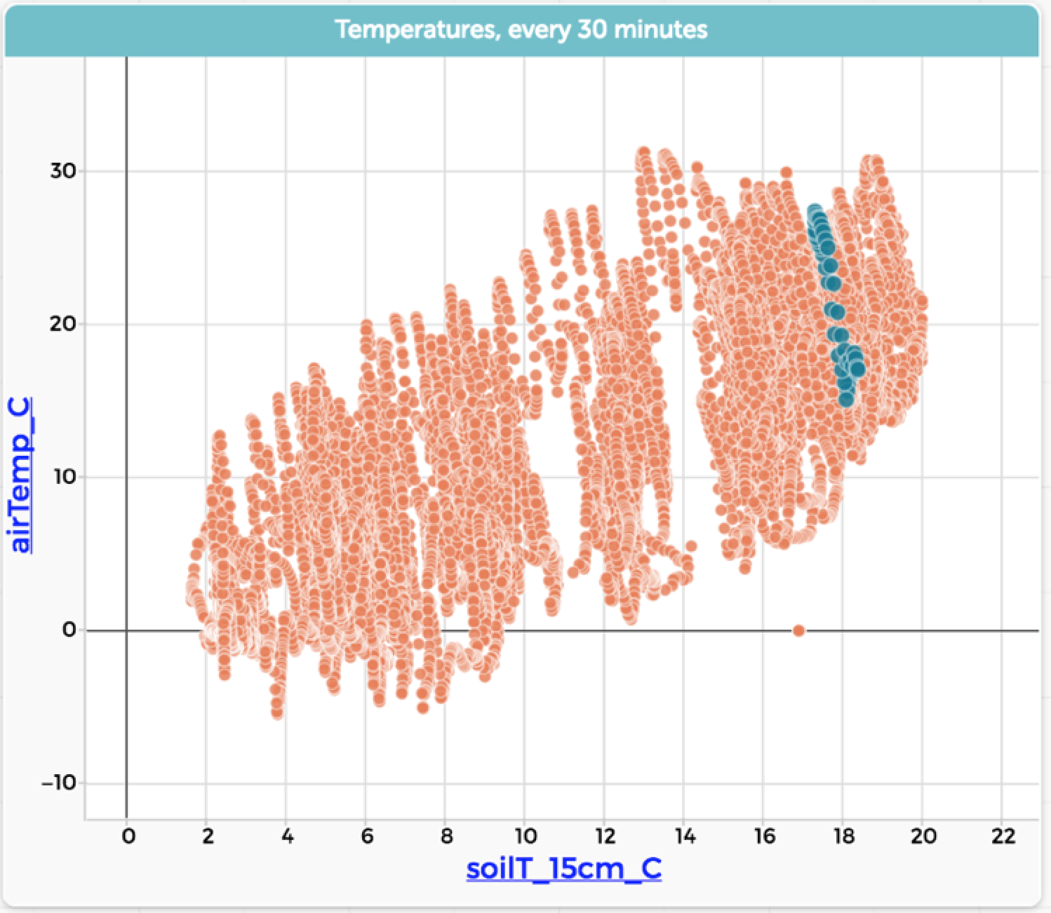
Now we do a “Hide unselected cases”—that is, filter the data to show only that one day—and rescale the graph:

Wow. What a difference. Looking at this graph, we see a much more detailed story from the data.

At the moment, in CODAP, this only works for graphs. You can’t, for example, filter a table to show only that one day; you have to actually delete the cases you don’t want to see. Maybe this will change.

select

Suppose you have a dataset in R—a table—with many variables, many columns. This function lets you make a copy of the table with only the columns you want. So this is not about selecting cases (rows) as we did in CODAP above.

CODAP does not have an equivalent of this function built in, but (as of 2021) there is a plugin called choosy that lets you hide attributes (columns) without deleting them. That plugin has other cool features as well; check it out!

arrange

In R, “use desc to sort a variable in descending order.” CODAP (finally!) has a sort capability as a menu item in the table.

Wrap-up

So it seems that, on the surface at least, CODAP can mimic a lot of the basic functionality that you will find in dplyr. There is a lot more to the package than we have discussed here, but if dplyr is a grammar of data manipulation, something like CODAP can at least order a meal and find a laundromat.

I’m not trying to say that you (or Rob Gould) should use CODAP instead of R. Sure, you can do cool things by dragging in CODAP that you have to do by remembering syntax in R. But R is a programming language, and you (for now, anyway) need all that syntax in order to express the things that you want to do in a save-able, repeatable, modular sequence of operations.

But wouldn’t it be great if before they had to learn the syntax, students understood why filtering is a good idea? Or what it means to compute some aggregate value?

And frankly, dear readers, how many times have we all tried to learn some new programming or data-analysis system? Given my tiny mind, at least, I have a devil of a time making that first scatter plot or drawing that first blue rectangle on the screen. Sure, once you know R Studio, it’s easy to do in R Studio. But how many people give up in those first few hours, or don’t give up but never quite know what’s going on? Maybe CODAP, or something like it, is a path to getting more people to stick around long enough to see how cool this all is.